The Inside Story of ClickHouse (1) Data Storage and Filtering Mechanisms

This article mainly discusses the data storage structure in ClickHouse, including file organization and indexing structures, as well as the data filtering mechanisms built on top of them. These mechanisms range from part pruning to mark pruning, and finally to SIMD-based row filtering.

The data filtering mechanism is essentially an algorithm built on top of the data storage format. Therefore, before introducing the filtering mechanism, we will first introduce the data storage format in ClickHouse.

PS: This article is based on ClickHouse v24.1

1. Directory Structure of Data Storage

ClickHouse adopts a common partitioning method used in big data systems for its directory structure of data storage. Within each partition, the data is further subdivided into files.

The data in a table is first divided into multiple partitions based on a partition key, which is often a date. For example, in the diagram below, the data is partitioned by month. Each batch of data insertion forms a smallest storage unit, which is called a Part in ClickHouse. Each Part belongs to a specific partition.

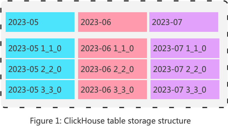
In ClickHouse, all Parts of all partitions of a table are placed in the same directory. The partition to which a Part belongs can be distinguished by the Part’s name. The naming convention for Parts is as follows:

partition-id _ min-id _ max-id _ level

The internal file organization within a Part directory is as follows:

1. primary.idx – This is the primary key index file, which records the primary key index value corresponding to each Mark. There is one .idx file for the entire dataset.
2. [Column].mrk – This file records the offset of the data in the data file (.bin file) corresponding to each Mark (introduced in the index structure section). Each column has a .mrk file.
3. [Column].bin – This is the actual data file. Each column has a .bin file.
4. checksums.txt – This is the part checksum file, used to verify data integrity.
5. columns.txt – This metadata file records the column names and data types.
6. count.txt – This metadata file records the total number of rows in the Part, which can be used to speed up count(*) queries.
7. partition.dat – This file contains the partition expression.
8. minmax_[Column].idx – This file contains the minimum and maximum values of a specific column, which can be used to speed up queries. The partition key always has a minimum and maximum index for partition pruning.
9. statistics_(column_name).stat – This file contains statistical information about a column, used to accelerate queries.

2. Index Structure

Each part forms a complete index structure. Overall, ClickHouse storage is columnar, with each column stored separately (in compact mode, multiple files are merged into one, but the essence remains the same). The general idea behind ClickHouse indexing is as follows: first, the entire dataset is sorted based on the indexed columns, similar to MySQL’s composite index; then, from the sorted data, one row is selected every 8192 rows, recording its index value and sequence number, forming a sparse index. This sequence number in ClickHouse is referred to as a Mark, meaning a Mark represents a group of data.

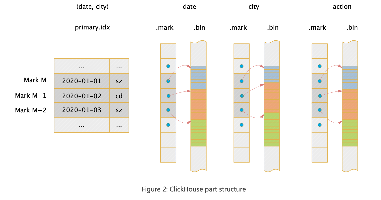
The following diagram illustrates the index structure of a two-dimensional table (date, city, action), where (date, city) are the indexed columns. The macro structure of the entire part file is as follows:

So how does a query use the index? Let’s take the following query as an example:

select count(distinct action) where date=toDate(2020-01-01) and city=’bj’

1. Locate the primary.idx and find the corresponding set of Marks (i.e., data block sets).
2. For each column to be read, use the .mrk file to locate the offset of the data in the .bin file corresponding to the Mark.
3. Read the corresponding data for subsequent calculations.

The above are the macro steps; the specific principles will be introduced below.

3. When to Use Indexes

During the SQL compilation phase, when initializing the execution pipeline, ClickHouse analyzes the data to be queried. The goal is to determine which Marks from which Parts need to be read. The parsing result is represented by an AnalysisResult. When execution actually takes place, the Scan operator directly reads the data corresponding to these Mark lists.

    struct AnalysisResult
    {
        RangesInDataParts parts_with_ranges;	// The final list of Parts to be scanned, as well as the scan range for each Part.
        Names column_names_to_read;	                     // columns to read
        
        // the following are some statistics	
        UInt64 total_parts = 0;		// total count of parts
        UInt64 selected_parts = 0;		// Number of Parts Hit
        UInt64 selected_ranges = 0;		// Number of Ranges Hit
        UInt64 selected_marks = 0;		// Number of Marks Hit
        UInt64 selected_rows = 0;		// Number of Rows Hit
    };

Key call stack:

ReadFromMergeTree::selectRangesToRead
ReadFromMergeTree::getAnalysisResult()
ReadFromMergeTree::initializePipeline
QueryPlan::buildQueryPipeline
InterpreterSelectWithUnionQuery::execute() 
executeQuery

4. KeyCondition

Before introducing how to use indexes, let’s first introduce its core algorithm, KeyCondition. The semantics provided by KeyCondition is to check whether a range matrix can satisfy the filtering conditions. When constructing KeyCondition, there are two necessary parameters: one is the syntax tree of the filtering condition, which is the main body of the filter, and the other is keys, which indicates that only these columns are concerned when determining whether the condition is met. Then, when using KeyCondition, the user needs to pass in a range matrix of keys to determine whether the range matrix satisfies the filtering conditions.

A range matrix is an array of ranges for the keys. For example, a range matrix composed of three primary key columns c1, c2, and c3 can be [[a, b], [1, 1], [x, x]]. When the user performs Mark pruning, a range matrix is generated and then it is determined whether this range matrix meets the conditions. Another example is a commonly used time partition range matrix, which can be [[2023-11-22, 2023-11-22]]. When the user performs partition pruning, each partition is traversed to construct a range matrix, and then it is determined whether the partition meets the conditions.

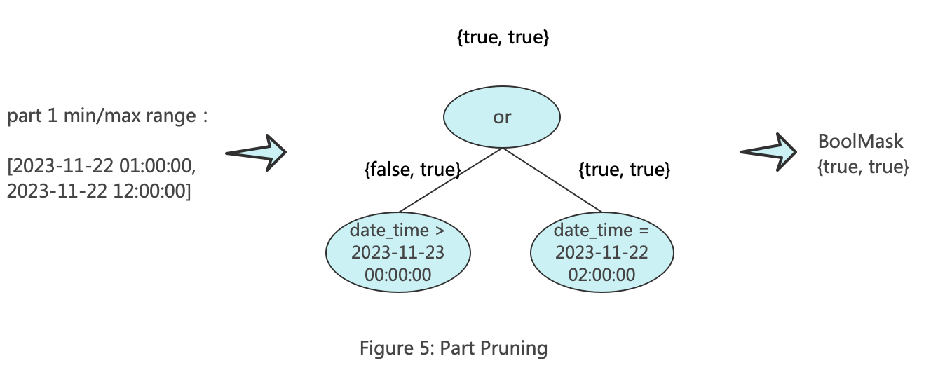
There are three cases for meeting the filtering conditions: 1. all data in the range matrix satisfies the filtering conditions, 2. some satisfy, 3. none satisfy. To represent the above three semantics, ClickHouse sets a data structure BoolMask {can_be_true, can_be_false}, where its {true, false}, {true, true}, and {false, true} values correspond to the above three semantics.

The core of KeyCondition is the RPN (Reverse Polish Notation) expression. Compared to infix or other notations, the advantage of RPN is its simplicity in computation. During calculation, a stack is used, and when an operator is encountered, operands are popped from the top of the stack to complete the sub-expression calculation, thereby completing the entire expression calculation.

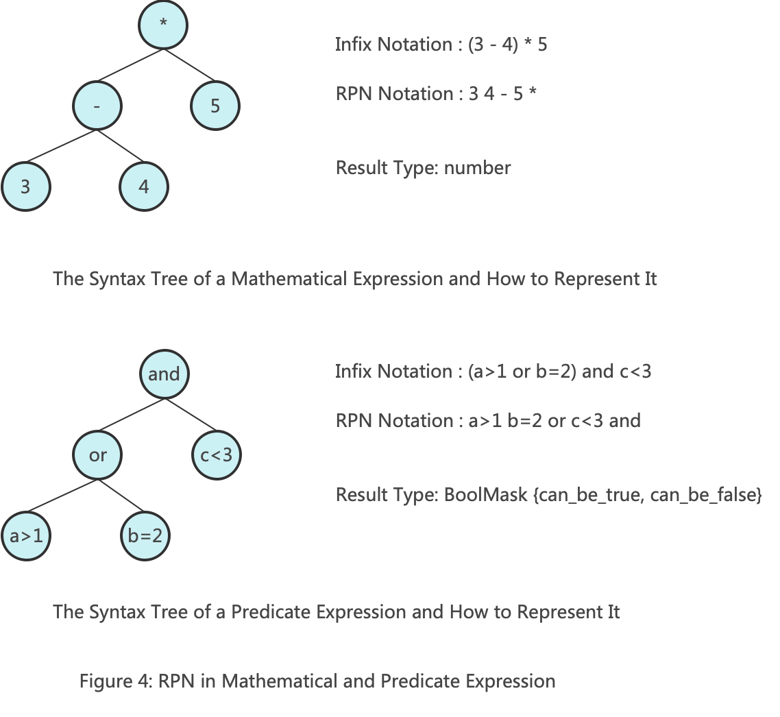
By using an analogy, we can better understand how RPN is used in filtering scenarios. The diagram above shows the usage of RPN in both arithmetic operations and filtering scenarios. The only difference between the two scenarios is the result type: one is a number, and the other is a BoolMask {can_be_true, can_be_false}. For more information about RPN, please refer to the wiki.

5. How to Use Indexes

5.1 Part Pruning

The purpose of part pruning is to filter entire part files at once, retaining only the parts that may contain the target data. In the process of part pruning in ClickHouse, two KeyConditions are constructed. One of them is called minmax_idx_condition, which is primarily used for part filtering based on the maximum and minimum values of the partition columns. The keys of minmax_idx_condition are the original columns corresponding to the partition key. For example, if the partition key is toDate(date_time), then its key is the date_time column. When filtering later, the range matrix composed of the values corresponding to date_time is passed in. The diagram below illustrates the working principle of minmax_idx_condition.

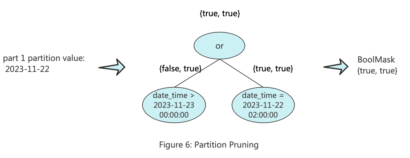
The other one is called partition_pruner, which is primarily used for partition filtering. The key of partition_pruner consists of the columns formed by the partition expression. For example, if the partition key is toDate(date_time), then its key is toDate(date_time). When filtering later, the range matrix composed of the values corresponding to the partition is passed in. The diagram below illustrates the working principle of partition_pruner.

The main logic of part pruning is located in: MergeTreeDataSelectExecutor::selectPartsToRead. You can refer to it yourself:

for (size_t i = 0; i < prev_parts.size(); ++i)
{
           if (!minmax_idx_condition->checkInHyperrectangle(        // Part pruning is performed based on the min-max index of the columns in the partition key.
                part->minmax_idx->hyperrectangle, minmax_columns_types).can_be_true)
            continue;

            if (partition_pruner->canBePruned(*part))	                   // Part pruning is performed based on the partition expression.
                continue;

            parts.push_back(prev_parts[i]);
}

5.2 Mark pruning

After filtering parts, mark filtering is further performed. First, let’s review what a mark is. Within a part, data is sorted according to the primary key, and then grouped every 8192 rows. This group ID is called a mark. A mark represents a group of data ordered by the primary key.

The smallest granularity of ClickHouse index filtering is a mark. The diagram below shows the data structure of a part with a primary key composed of columns c1, c2, and c3, as well as the process of mark filtering.

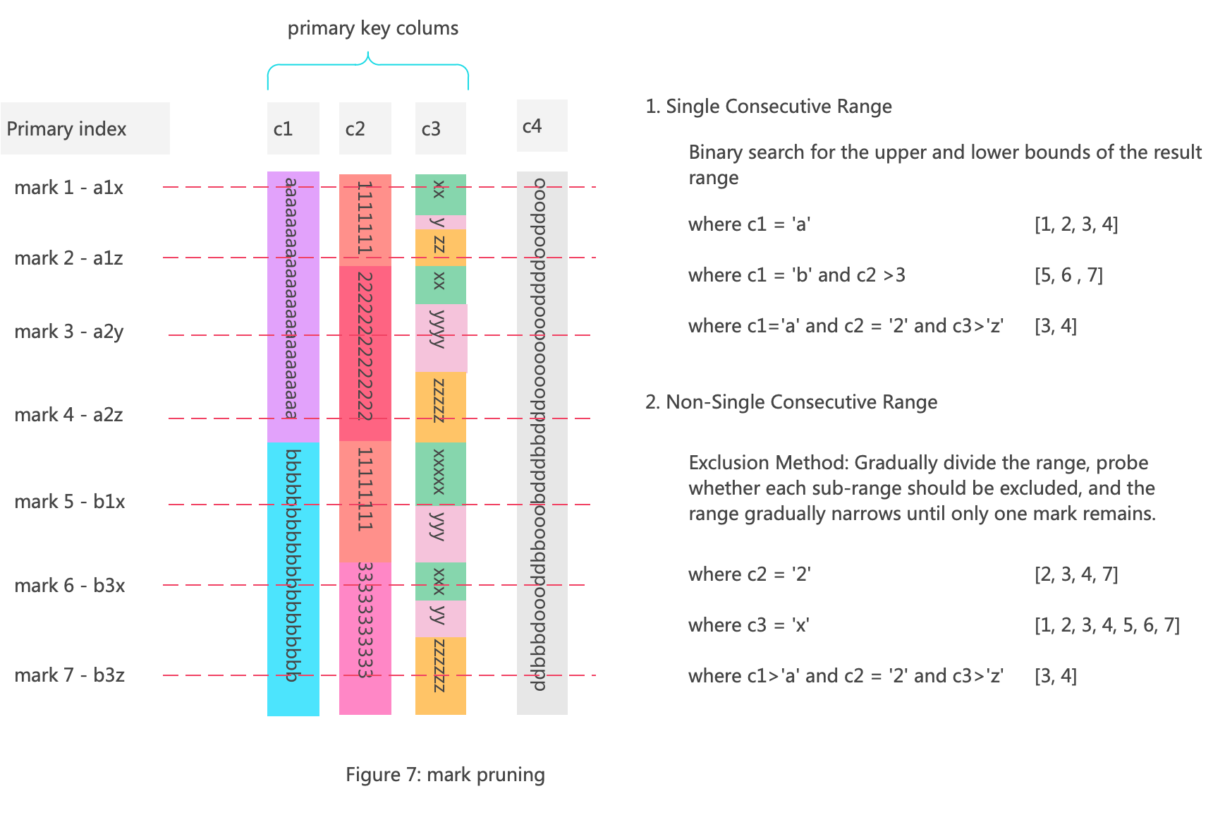
For a part file composed of continuous mark ranges from 1 to n, mark pruning involves removing sub-ranges that do not meet the query conditions.

If the mark ranges represented by the query condition is a single and continuous range, such as WHERE c1='a', then the pruning of marks can be done by using binary search to find the upper and lower bounds of this single range.

If it is not a single continuous range, such as WHERE c2='2', then the exclusion method is used. This involves gradually dividing the mark range and excluding sub-ranges that do not meet the conditions.

During the mark pruning process, the input is a MarkRange, for example, [2, 5], and the output is a series of MarkRanges. So, how do we use KeyCondition in this context?

Since KeyCondition performs judgment based on the range matrix of the primary key columns, it is necessary to first convert the MarkRange into a range matrix. Converting a MarkRange into a range matrix is akin to converting a range in a multi-dimensional space into a range in a one-dimensional space. Therefore, the resulting range matrix might have multiple representations. This discussion will not delve too deeply into this aspect, but for those interested, you can refer to the KeyCondition::forAnyHyperrectangle method.

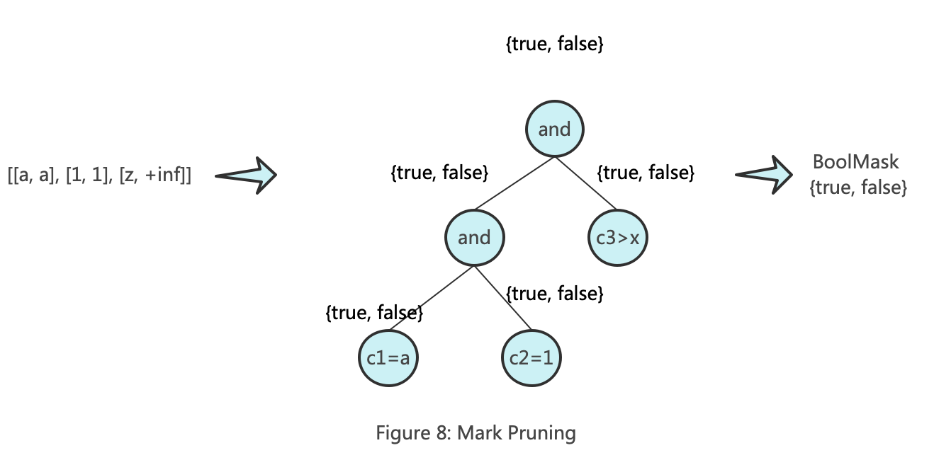
One of the range matrices converted from MarkRange [2, 5] could be [[a, a], [1, 1], [z, +inf]]. The diagram below illustrates the working principle of KeyCondition in pruning marks:

At this point, we have filtered out a series of marks, and the mission of the data storage structure and index in the filtering process is complete. Next, we need to filter the rows within each mark.

6. Row Filtering

Row Filtering occurs during the query execution phase. In ClickHouse, Row filtering is also performed in a batch manner. This batch is internally referred to as a Chunk in ClickHouse, and its size may differ from that of a Mark. The primary logic for filtering numeric type columns is recorded in ColumnVector::filter (the filtering logic for other column types is similar).

6.1 Generate Filter Mask:

First, generate a Filter Mask for a Chunk of data based on the filtering conditions. The Filter Mask is a UInt8 array with a length equal to the number of rows in the Chunk. This array contains only two values: 0 indicates that the row does not meet the filtering conditions, and 1 indicates that it does.

6.2 Filter column by Filter Mask：

Filter data based on the Filter Mask. The filtering process is optimized using SIMD technology. The specific process is as follows:

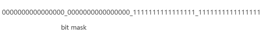
First, data is grouped and processed in chunks of 64. Then, the byte mask is converted into a bit mask. Refer to the function bytes64MaskToBits64Mask. The converted bit mask can be directly represented by a single UInt64.

For each group, filter according to the different data distribution scenarios:

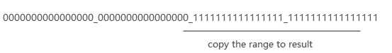
1. If bit_mask equals 0, meaning the bit mask for this group is all zeros, directly ignore this group.
2. If bit_mask is all ones, copy the entire group to the result set.
3. For mixed patterns such as [0]+[1]+ or [1]+[0]+, copy the continuous segments of ones in the byte mask to the result set.

6.3 Filter column by Filter Mask version 2

For the filtering part, ClickHouse provides a SIMD version (using the AVX512 instruction set). Data is still grouped and processed in chunks of 64. Then, the byte mask is converted into a bit mask. Each group is processed according to the different data distribution scenarios.

1) If the bit mask is all zeros, directly ignore this group.

2) If the bit mask is all ones, copy the entire group to the result set using vectorized methods for batch copying.

_mm512_storeu_si512(reinterpret_cast(&res_data[current_offset + i]), 
               _mm512_loadu_si512(reinterpret_cast(data_pos + i)));

3) For other cases, use the vectorized function _mm512_mask_compressstoreu_epi8 to copy data to the result set according to the mask.

6.4 Filtering the tail part.

6.5 Summary of Row Filtering Optimization

1. Why Use Filter Mask?

1. When filtering multiple columns, the Filter Mask can be reused.
2. It facilitates the use of SIMD instructions.

2. Why Process in Groups?

Because ClickHouse sorts data by primary key, in many cases, data is locally ordered by certain columns. This allows for entire groups to be filtered out or hit with a high probability during filtering. Compared to processing individual rows, this approach eliminates the need for conditional checks during processing, thus avoiding branch prediction failures and preventing CPU pipeline disruptions. It also increases the hit rate of instruction and data caches, which is a core design point for high-performance filtering.

3. Is It Always Better to Use Wider SIMD Instruction Sets, Such as AVX512 Over SSE2?

In most cases, yes, but not in filtering scenarios. Increasing the width also increases the group size. The larger the group, the smaller the probability of having all zeros or all ones in the group, thus reducing the likelihood of filtering out the entire group. Therefore, it depends on the data distribution.

This work is licensed under a Creative Commons Attribution 4.0 International License. When redistributing, please include the original link.