ClickHouse is an outstanding OLAP product that has led the industry trend towards vectorized execution engines. It excels in many areas, particularly in the optimization of underlying data structures and algorithms, as well as in the richness of its features. However, it falls short in terms of its optimizer. To address this, the team has developed the ClickHouse Cost-Based Optimizer (CBO) with the goal of further enhancing ClickHouse’s performance.
1. Optimization Effects
We used ClickHouse’s ClickBench for our testing, with a dataset of 100 million rows. The testing environment consisted of a 5-node ClickHouse cluster with a single replica. Each node had the following specifications: 32 cores, 128 GB of RAM, and 1 TB of NVMe storage.
The benchmarking method involved running each query from the list three times, both with the CBO optimizer enabled and disabled. The benchmark results are as follows:
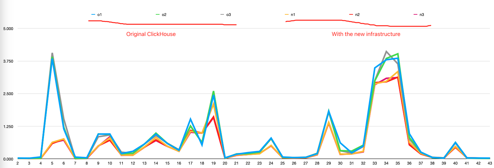
With the CBO optimizer enabled, some queries showed significant improvement. The total query time for 43 SQL queries decreased from 32 seconds to 22 seconds.
Note: The ClickBench list consists of queries with single-table aggregations, which are relatively simple. In multi-table scenarios, it is expected that the CBO optimizer will have an even more pronounced impact on performance.
2. Why we need an optimizer?
In the spirit of “a single example is worth a thousand words,” we will use two queries (examples) to illustrate.
2.1 query_1
select a,b,c from t1 inner join t2 on t1.id=t2.id where t1.d='xx'Assuming a cluster with 100 nodes, with tables t1 and t2 containing 1 billion rows and 100 rows of data respectively, the execution plan for query_1 is as follows:
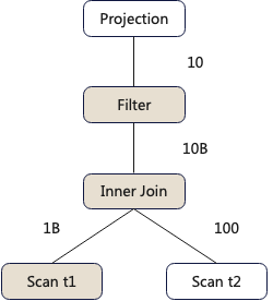
PS: In the diagram, the squares represent operators, and the numbers on the lines represent the data output by the operator below. For example, after an Inner Join, 10 billion rows of data are output.
If we want to improve query performance, how can we optimize it?
1.Rule-based equivalent transformations
We can push the Filter operator down below the Inner Join, filtering in advance so that the amount of data that the Inner Join needs to compute changes from the previous 1 billion + 100 to 2 + 100.
2.Choosing the appropriate algorithm
The Inner Join in query_1 is the most performance-consuming operator, so optimizing it has a significant impact on the overall query performance.
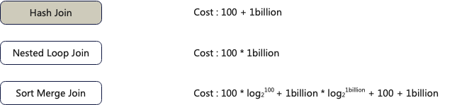
We can see that different algorithms have orders of magnitude differences in data computation costs. Here, we chose the Hash Join algorithm.
- Operator data distribution properties
Data distribution properties refer to how the algorithm of the lower-level operator distributes data to the upper-level operator. This optimization method is mainly used in distributed databases. Assuming the cluster for query_1 has a total of 100 nodes, there are 2 ways to distribute data for the operators below the Inner Join.
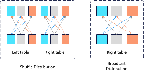
For the shuffle distribution method, 1 billion rows need to be transmitted over the network, whereas for the broadcast method, 100 * 100 rows need to be transmitted. Therefore, the broadcast data distribution method is more optimal here.
2.2 query_2
Let’s look at another example and how to optimize it.
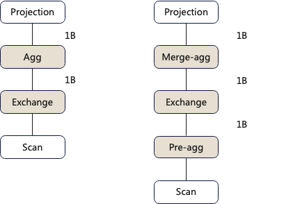
select a, sum(b) from t1 group by aIn the figure below, the left side shows the query plan, and the right side shows the optimized execution plan.

The difference between the two execution plans lies in the aggregation operator’s algorithm. The execution plan on the left uses a single-stage aggregation method, where the data scanned is directly sent to a single node for aggregation. The optimized execution plan on the right uses a two-stage aggregation method, where each node first performs an initial aggregation, and then sends the initially aggregated results to a single node for a second aggregation.
The amount of data transmitted over the network by the Exchange operator for the two different algorithms is 1 billion and 1,000, respectively. Clearly, the algorithm on the right is more optimal.
From the above two examples, we can see that SQL, as a programming language, only tells us what to do, but not how to do it. Different approaches can have a significant impact on performance, which is why we need an optimizer to choose the appropriate execution plan.
3. Why we need a CBO Optimizer?
In the above two examples, a series of optimization measures were provided, but these optimizations were derived from an omniscient perspective. In reality, we don’t know the output data volume of each operator, nor do we understand the computational cost of each operator. When the data characteristics differ, how do we choose different execution plans?
1. Assuming the input of the Inner-join in query_1 is ordered, which algorithm should be chosen?
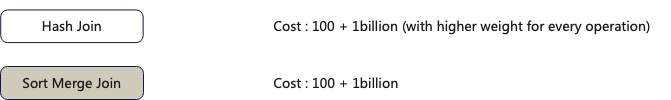
Based on the different computational costs of the two algorithms, the Sort-Merge algorithm is more suitable in this case.
2. Assuming the datasets in the Inner-join of query_1 are very large, how should the data be distributed?

For example, if both the left and right tables have 1 billion rows, the shuffle distribution method would require network transmission of approximately 2 billion rows, whereas the broadcast method would require network transmission of approximately 100 nodes * 1 billion rows = 100 billion rows. In this case, the shuffle distribution method is more suitable.
3. Assuming the cardinality of the data in query_2 is particularly large, how should the aggregation method be chosen?
For example, if the cardinality of the data is 1 billion, the network transmission cost for the Exchange in the one-stage aggregation method on the left execution plan is 1 billion, and the aggregation cost is 1 billion. For the two-stage aggregation method on the right execution plan, the network transmission cost for the Exchange is 1 billion, and the aggregation cost is 2 billion. Clearly, in this case, choosing the one-stage execution plan on the left is more suitable.
In summary, some optimizations are heavily dependent on data characteristics (data size, cardinality, sorting properties, data distribution), which is why a Cost-Based Optimizer (CBO) that optimizes based on data characteristics is needed.
4. How to use it?
Currently, we have submitted a PR to the community. If you are interested, you can compile it yourself. When performing queries, you can enable the CBO optimizer feature by turning on the switch allow_experimental_query_coordination.
Below is the detailed usage documentation:
1. Collect statistics
ANALYZE TABLE hits;2.Show query plan explanation
SELECT * FROM hits SETTINGS allow_experimental_query_coordination=1;3.Explain with statistics
EXPLAIN STATISTICS=1 SELECT * FROM hits SETTINGS allow_experimental_query_coordination=1;4. Explain with cost
EXPLAIN COST=1 SELECT * FROM hits SETTINGS allow_experimental_query_coordination=1;5. Show distributed query plan
EXPLAIN FRAGMENT SELECT * FROM hits SETTINGS allow_experimental_query_coordination=1;6. Set a hint to prefer using two-stage aggregation
EXPLAIN FRAGMENT SELECT OS, COUNT(*) FROM hits GROUP BY OS SETTINGS allow_experimental_query_coordination=1, cbo_aggregating_mode='two_stage';7.Show pipeline
Not implemented.
This work is licensed under a Creative Commons Attribution 4.0 International License. When redistributing, please include the original link.